Optical microscopes (microscopes using visible light as a medium) are limited by their resolving power, setting a minimum length between two points that can be differentiated. For a long time this has limited us to specimens above the size range of 0.2 micrometres (about half of the wavelength of light). Although cells, bacteria and some cell organelles can be resolved, proteins and small molecules were outside the bounds of this technique. This has overall greatly limited our microscopic methods. It was Abbe in 1873 who first noted the above limitation on resolution and hence the underlying limit to light microscopy bears his name.
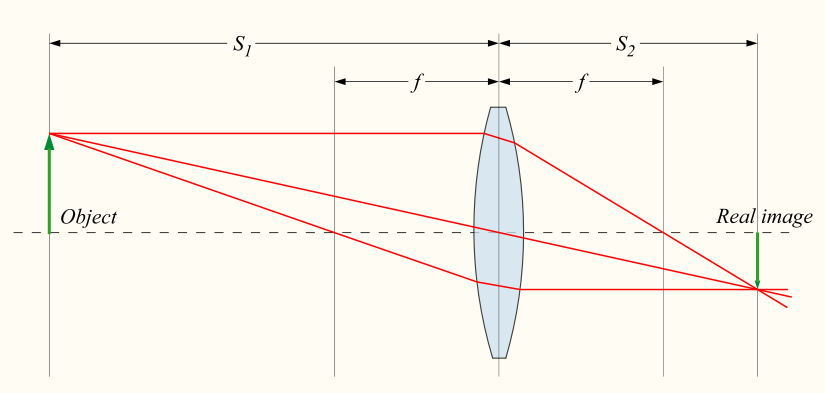
Below I will outline the geometric considerations leading us to Abbe’s limit on resolving power. The geometric method is chosen for its simplicity and ease of presentation. Imagine rays of light from a source travelling through the specimen into the lens. For a given microscope set-up we are asking, what the minimum distance between two points that can be seen through our objective is. In order for an image to be created by the light travelling through the lens, at least two beams of light have to coincide (at the point of focus). A single light beam is not enough to create a focused image. This is shown in the Figure 1 below.
It simplifies our approach (without losing meaning) to think
of the above set-up as a light beam traveling through a slit (the sample).
Now the question becomes: how small is the smallest distance (\(d_{min}\)) between two
slits such that we can still tell them apart.
We will find \(d_{min}\) on the sample when one of the light rays
is hitting the edge of the lens. This will be the ray that for any two points
maximises the angle at which the rays arrive and hence minimises \(d_{min}\).
The below diagram details the case when a ray is hitting the edge of the lens.
Here a ray of light is built from multiple waves (\(l_1, l_2\)) arriving from
different slits.
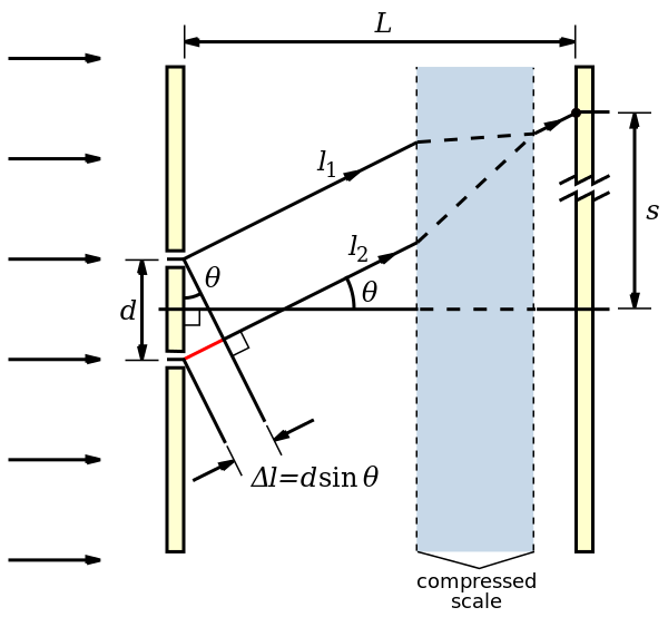
This is the limiting case (as the ray is hitting the edge of the lense),
and the two waves (\(l_1, l_2\)) combined
will form a coherent light beam. Moreover this will be the first diffraction
maxima (if there was another diffraction maxima before this that would mean
we could make \(d_{min}\) even smaller until we find the first diffraction maxima just
hitting the edge of the lense). This means the difference in distances
travelled between the two waves will be \(\lambda\) as this is the first diffraction maxima.
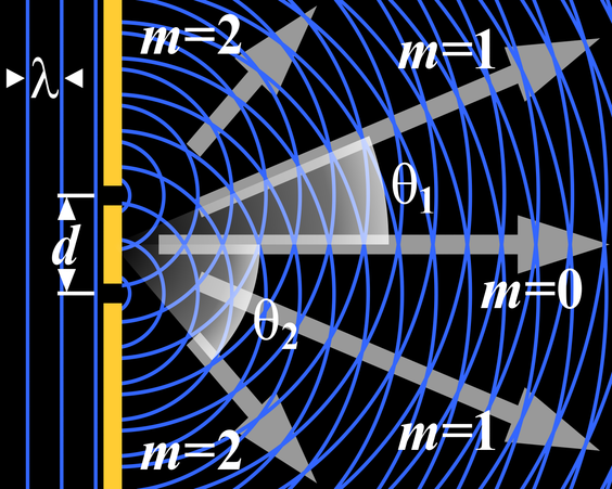
We can see this in action in the Fig.3 and corresponding animation Fig.4.
In the picture the slits are the wave sources. While the animation shows
the now combined waves forming diffraction maxima.
We can now look at how this condition informs the resolving power. Let’s
look back at Fig.2 geometrically. Fundamentally we want a geometrical connection
between the minimum distance,\(d_{min}\), and the other known properties
of the set-up, in order to put a lower bound on this distance.
With this we can derive the travel distance between two waves forming the
first diffraction maxima: \(\Delta l = d \sin \theta \) (Due to the right
angled triangle and \(\theta\)).
Further, as these waves are coherent the difference in distance travelled
will be \(\lambda\).
Now we know \(\Delta l = d \sin \theta = \lambda\) giving a relation between
\(\lambda\) wavelength and the angle \(\theta\).
This is the sort of connection between known quantities and \(d_{min}\) we
were looking for.
There is one more thing to iron out before we arrive at
Abbe’s formula.
In this case we are referring to the \(\lambda\) that is present between
the sample and the lens (this might not be the same wavelength as in normal
conditions). The new wavelength can be written as depending on the refractive
index of the material according to
Snell-Descartes law
that is present between the sample and the lens (this might not be the same wavelength
as in normal conditions). This will give us the final connection we were
looking for.
For a wave passing from one medium to the next the following
holds for the refractive index:
\(n_{2,1}=\frac{n_2}{n_2}=\frac{c_1}{c_2}=\frac{\lambda_1 f}{\lambda_2 f}=\frac{\lambda_2}{\lambda_1}\)
where \(n,c,f\) are the refractive index, the
ray's speed and the frequency for the given medium.
Let’s further simplify this for when the first medium is vacuum:
\(\frac{n_2}{1}=\frac{\lambda_1}{\lambda_2}\) and \(\lambda_2 = \frac{\lambda_1}{n_2}\).
Now we can put this back into the first eqn to get the relation between
the wavelength of the outside medium to the angle within
\(\frac{\lambda_1}{n_2} =d \sin\theta \).
And we arrive at \(d = \frac{\lambda_1}{n_2 \sin\theta}\).
Last we need to introduce a scaling factor of 0.61 due to properties of the lens:
\(d = 0.61\frac{\lambda_1}{n_2 \sin \theta}\)
here \(d\) is the resolving power (smallest distance that can be resolved)
\(\lambda_2\) the wavelength in vacuum
\(n_2\) refractive index of the material between the lens and the sample
\(\theta\) aperture of the lense
\(n\sin\theta\) is the numerical aperture.
Finally we have Abbe's limiting factor \(d = 0.61\frac{\lambda_1}{n_2 \sin \theta}\).
As we see above, this equation has described the fundamental limit to light
microscopy that has been present ever since its invention. Abbe's limiting
factor is the closest there is to having a physical limit to light microscopy.
To put it simply it says the shorter the wavelength the better the resolution
of the microscope. This is why in the next section X-rays and electron microscopes
both with shorter wavelengths are introduced for resolving power.
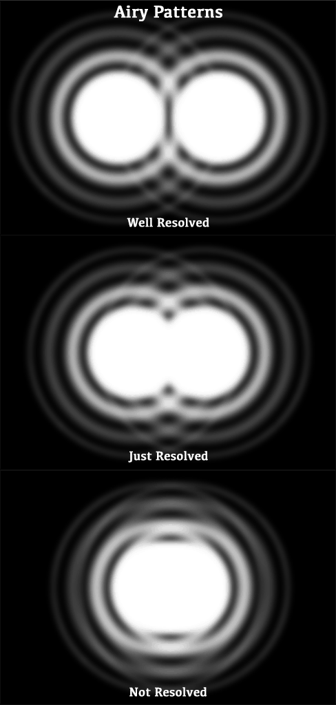
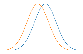
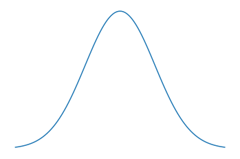
As we can simply approximate the waves leaving a point as a Gaussian distribution, if two points are close to each other the Guassians will have large parts of their distribution overlapping. Whereas if two points are sufficiently far from each other (outside the resolving power distance) the distribution will be easy to tell apart. So if we go above the resolving power of a microscope we will not be able to differentiate between two points. In Fig.5 the top two signals are well resolved, while the one at the bottom is not. The lowermost signal can be thought of as two Gaussians with very similar means. And in Fig.6 and Fig.7 we see two signals that are not resolved well and a signal that is well resolved represented as a dsitribution.
As the resolving power of light microscopy has been fundamentally limited, there have been various alternative ways of looking at small distances.
This technique uses light microscopes with oil between the sample and the objective. This gets around Abbe's limit by changing the refractive index \(n_2\) in the eqn \(d = 0.61\frac{\lambda_1}{n_2 \sin \theta}\). If the refractive index is increased (and is above 1), we can see the minimum distance between two points that can be resolved will decrease. Oil has a refractive index of 1.515, hence a decreased minimum resolution distance and increased power. However this will only have 1.515 higher resolving power, leaving us still uncapable of looking at cell structure.
The electromagnetic waves are X-rays, meaning the small wavelength allows a higher resolving power. However, it relies on X-ray diffraction and Bragg’s law, so they can be only used on crystallised materials. Meaning living cells and organisms can’t be used. This is a major limitation. Nevertheless, X-ray crystallography was used in the experiments performed under the supervision of Rosalind Franklin to image DNA, providing crucial evidence for the helical structure of Watson and Crick’s model with the backbone being on the outside.
Here electrons are used for reflecting off our sample, again these have a higher frequency and shorter wavelength (shorter by \(10^{-5}\)) than the visible light spectrum. This results in 100x the resolving power compared to light microscopes Additionally, electron microscopes can be used on non-crystallised materials and have been crucial in determining the structure of cells. However, electron microscopes are not useful for imaging live cells, as specimens need to be prepared. This often means freezing, coating in metal or chemical fixation, all resulting in cell death.
Thanks to David Urban, Loren Kell, Kalman Lajko and Reka Tron for reviewing this.